Uncovering HR Data using Statistics: What Factors Impact Attrition?

Intro

Attrition is something that all companies experience and while the reasons for it can vary, it is important that those reasons aren’t ever related to inequality or discrimination in the workplace. Unfortunately, sometimes it can be unclear whether those aspects are at play, and looking at exploring data can help us find the answers. In this project I analyzed an HR Dataset from IBM to find whether relationships exist between attrition and various factors such as age, experience, and more. Using statistics along with linear and logistic regression in R, I found some answers to important questions:

Do older employees leave more than younger employees?
Are junior employees more likely to leave or be laid off than senior employees?
How does worklife balance affect employee length of stay?
Does job stagnation affect turnover rates?
How strongly can years of experience predict income?

Data Analysis

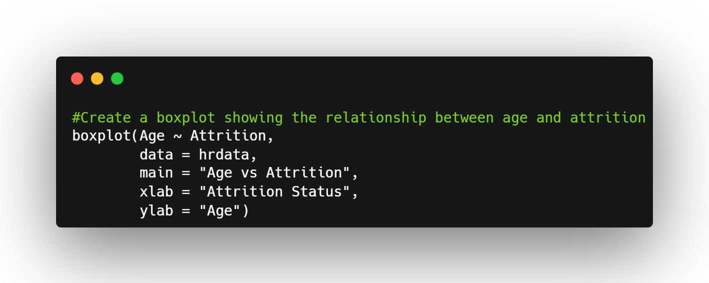
To begin my exploration, I started by looking for any potential ageism that might be happening at the company, specifically against older individuals. By creating a boxplot using the two variables of Age and Attrition, I was able to get a high level visual of their relationship.

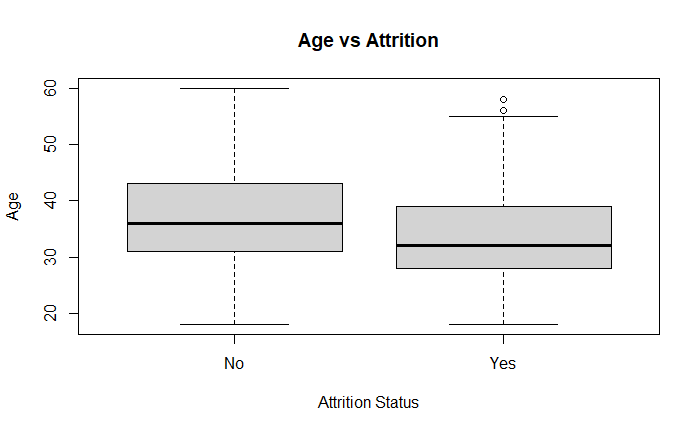At first glance, we can see that the Median Age for those who left is actually lower than the Age of those that didn’t.

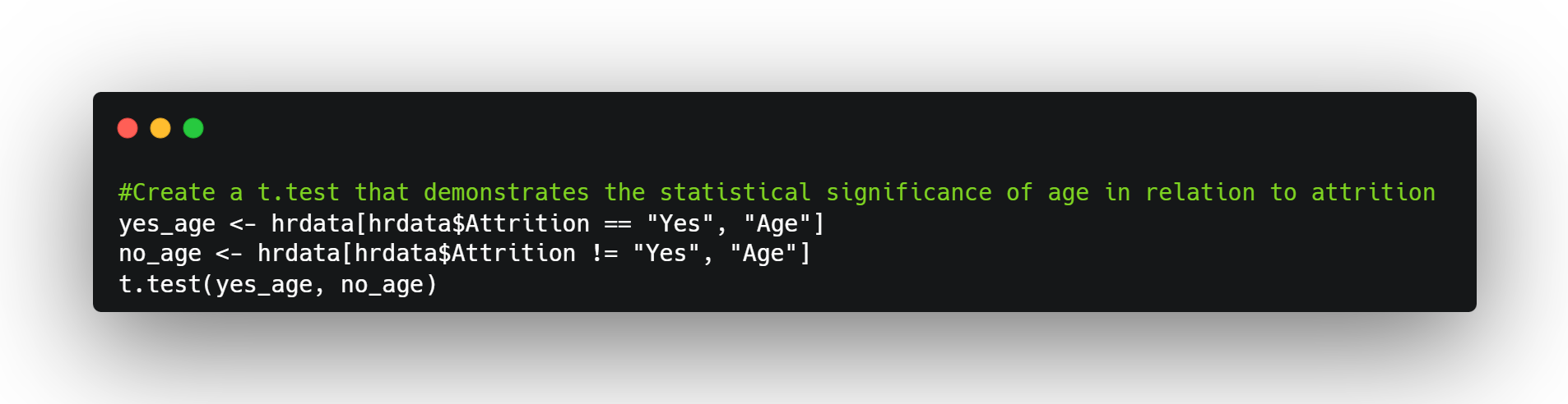
To get a more in-depth look at the difference between the two groups, (employees that turned over vs employees that didn’t turn over) I conducted a t-test to find out if there is a statistical significance. Before I could go through with this, I established variables that met the criteria for the two groups I wanted to test:

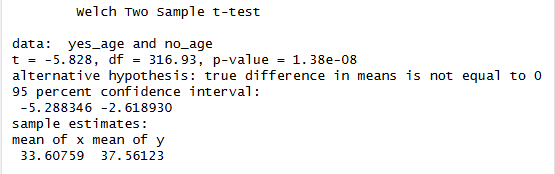
Once that was established, I performed the t-test below and got a clearer understanding of the difference. Because the p-value was less 0.0000000138, which is less than 0.05, this proved that there was a statistically significant difference between the two groups, although it was the opposite of what was being searched for. In actuality, the average age of those who left was about 34, younger than the average age of retained employees which was about 38. While it appears that younger employees are leaving more than older ones, we can see that the difference in the Mean between the two groups is not very big, which is a good sign that there seems to be minimal age discrimination.

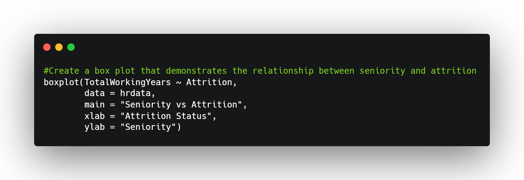
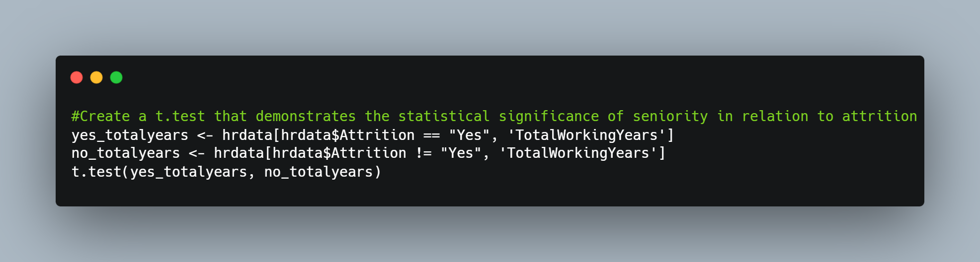
While knowing the significance of age in relation to attrition is a great start, another common concern within the turnover discussion is employee seniority. Using similar methods as before, I dove deeper into the variables of seniority and attrition to see how strong their relationship is. (In this instance, Employee Number represents level of seniority. Larger numbers are newer employees and smaller numbers represent tenured employees.)

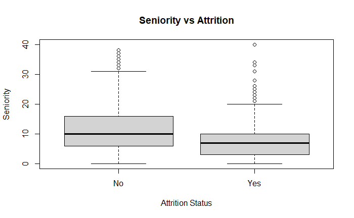
The initial visualization revealed that the Median between the two groups is slightly different and running a t-test here was especially helpful to see whether there was a statistically significant difference between the variables.

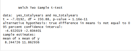
Not only did the t-test demonstrate how close the Means of the two groups were, but it established that the p-value was low at 0.0000000000116. This made it apparent that statistically, seniority is significantly related to turnover rate. Junior employees are in fact more likely to leave or be laid off than Senior employees. Nonetheless, it is important to acknowledge that in this dataset the similarity in the Means indicates that at IBM the difference is marginal.

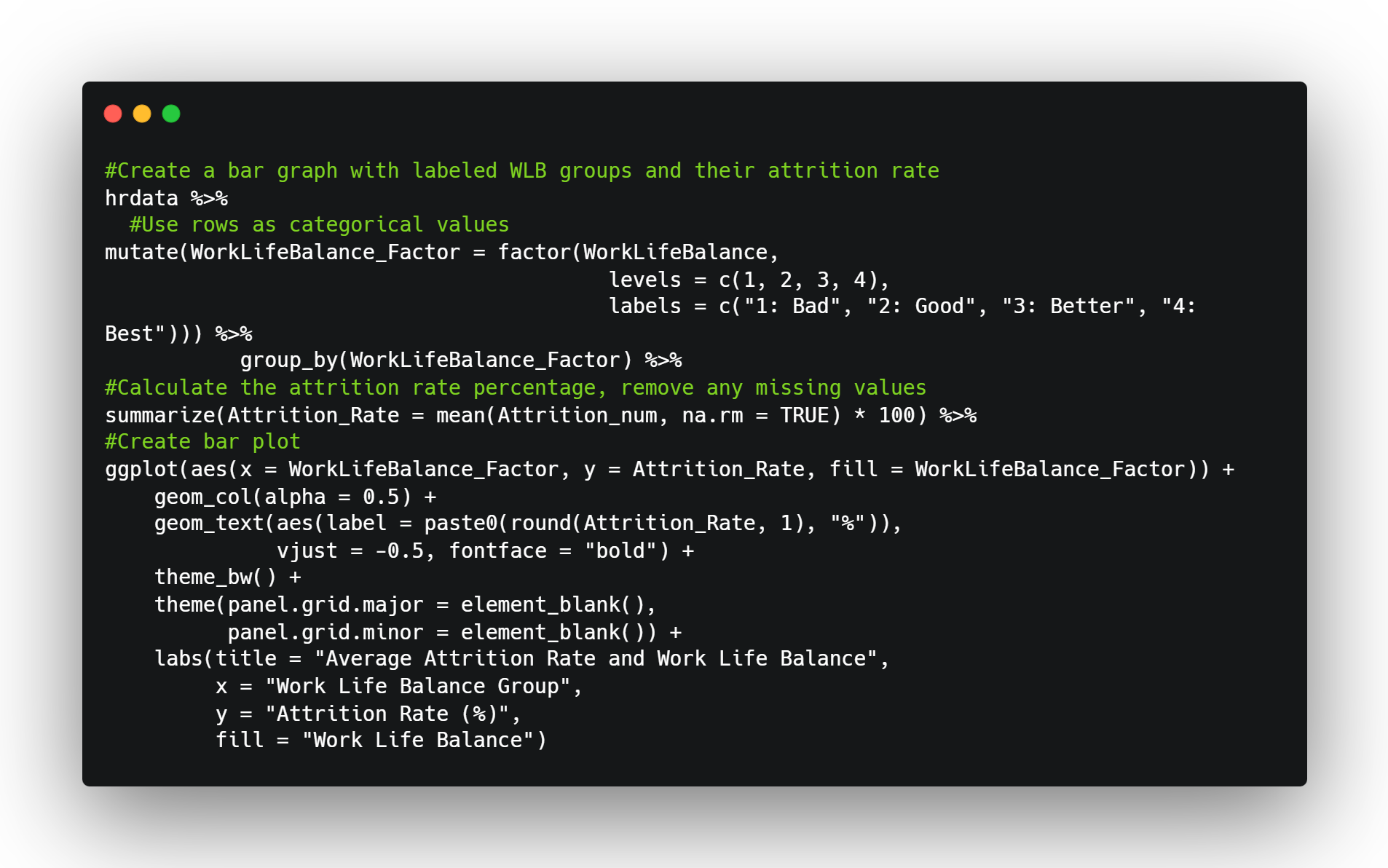
It has been great to find that there has been minimal discrimination in the attrition process when focused on the factors of age and seniority. That being said, something that can sometimes go unheard in the conversation is the importance of worklife balance. Worklife balance doesn’t look the same for everyone, and learning more about how it can affect an employee’s length of stay can be beneficial to an organization’s efforts towards reducing turnover rates. To learn more, I created detailed visualizations using the ggplot and pipe operator functions from the tidyverse library.

Within the dataset, the WorkLifeBalance column had rows labeled 1-4, with each number representing a category rather than a scalable number. Before creating the bar graph, I had to ensure that R knew to view these values as categories by creating a factor for WorkLifeBalance. In addition to this, I wanted to see the actual risk of attrition within each category, rather than just the count.

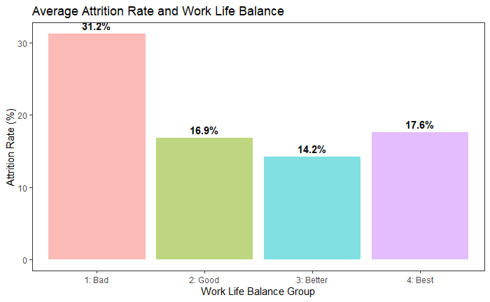
While a higher risk of attrition from the “Bad” worklife balance group might’ve been expected, the data implies that it’s actually true. I found it interesting that although the risk lowered as the worklife balance got better, there was actually a spike in risk when comparing the “Better” group to the “Best” group. This signals to the organization that although an enjoyable worklife balance can lessen the risk of employees leaving, it isn’t always the deciding factor. Additionally, they could conduct further investigation into sample size for ultimate certainty.

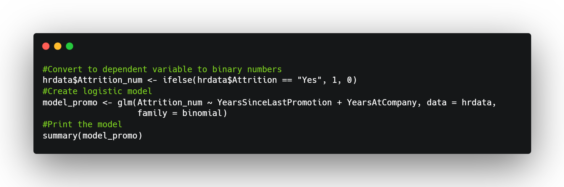
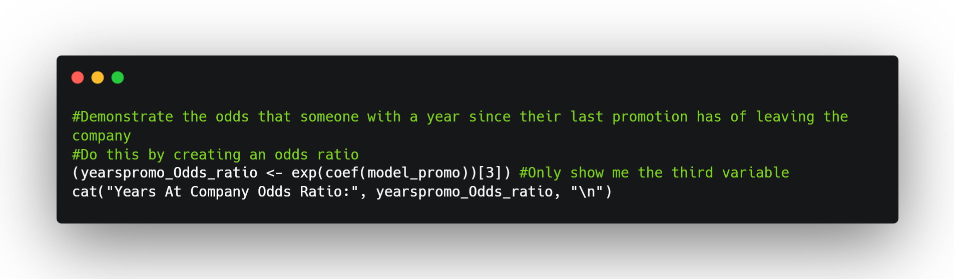
These results led me to find out more about the relationship between attrition and another factor: job stagnation. This is another variable that could be the final decision-maker for someone thinking about leaving a company. By using logistic regression, I was able to see how strongly YearsSinceLastPromotion can impact the likelihood of someone leaving by looking at the association between YearsSinceLastPromotion, YearsAtCompany, and Attrition.

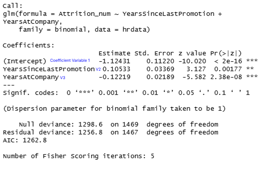Looking at the p-values above, it looks like both variables have a statistical significance. Once again, this is a good overview, but I decided to show their effect in the form of an odds ratio. The odds ratio can make it easier to understand the true impact of both variables.

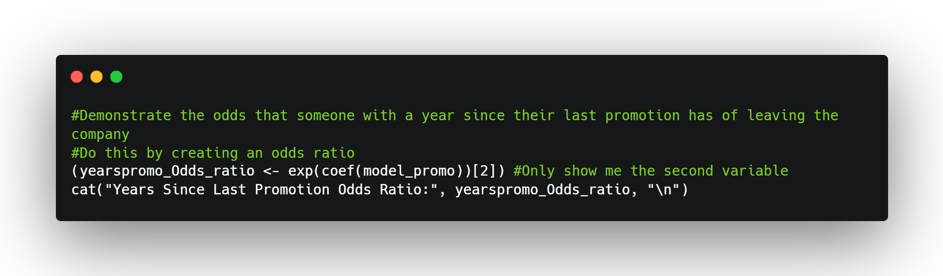
In the odds ratio for YearsSinceLastPromotion seen above, we can see that for every year that passes where an employee is not promoted, the odds of them leaving the company increase by 11%. This may not seem like a lot at first, but if for example an employee goes somewhere between 3-5 years without a promotion, the odds increase quickly. After five years, an employee’s odds of leaving could increase by 68%.

On the other hand, when we look at the Odds Ratio for YearsAtCompany, given the value is below 1, that tells us that the odds of someone leaving the company decrease by 11.5% after every additional year they spend at the company.

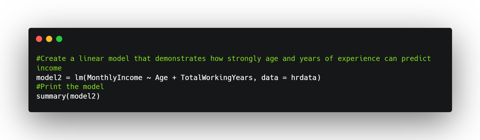
The final question to be answered was related to years of experience. After finding out how years without promotion can increase the odds of employee attrition, IBM could implement new promotion strategies by getting a better idea about how age and years of experience impact somebody’s income.

To do this, I used a linear regression model that looked at the association between the variables of Age, TotalWorkingYears, and MonthlyIncome.

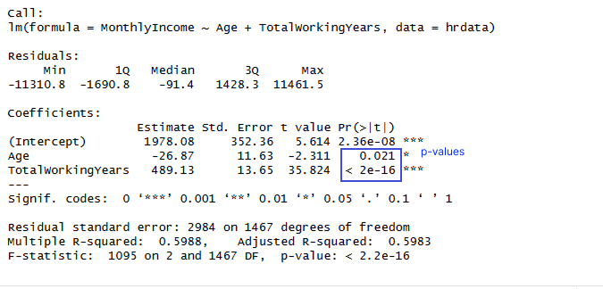The p-value for Age tells us that it is statistically significant in relation to MonthlyIncome because although it is higher than the p-value for TotalWorkingYears, it is still lower than the 0.05 significance threshold. Additionally, the p-value for TotalWorkingYears is also significant, with a value of less than 0.0000000000000002. While both TotalWorkingYears and Age are statistically significant indicators of MonthlyIncome, the R-squared value also establishes that roughly 60% of the total variance in MonthlyIncome can be collectively explained by both variables in the model.

Since years of experience are clearly a strong predictor of income, this suggests that IBM should ensure their promotion assessments are fair by keeping experience in mind to help prevent employee turnover.

Final Insights

Younger employees leave the company more often than older employees.
Junior employees are more likely to leave or be laid off than senior employees.
Worklife balance affects the risk of employee attrition. The worse the worklife balance is, the higher the risk of an employee leaving.
Every year an employee remains without a promotion in their current position, the odds of them leaving the company increase by 11%
Years of experience are a strong predictor of income, signaling the importance of fair promotion assessments.

This analysis revealed the importance of considering multiple factors when assessing employee attrition. By understanding how factors such as age, worklife balance, years of experience, and monthly income can increase or mitigate the risk of turnover, IBM can implement more nuanced strategies to reduce overall attrition.

Thank you for taking the time to check out my project! If you’d like to chat or have any questions, feel free to connect with me on LinkedIn!

Click here to checkout the original dataset used in this project.